Payback Maths On A Robot Cell
Origin and history
The analytical process known as "payback maths" for robot cell investment originated in the manufacturing industries of Western Europe and North America during the late 20th century. Its development coincided with the widespread adoption of programmable industrial robots in automotive and electronics assembly lines throughout the 1980s and 1990s. The methodology formalized earlier, ad-hoc capital budgeting techniques that factory managers used to justify the high upfront cost of automation. It evolved from basic return-on-investment calculations into a more nuanced model specific to robotic work cells. The framework became a standard part of industrial engineering and operations management curricula by the early 2000s. Its principles are now documented in professional handbooks and form a core component of feasibility studies for automation projects globally.
What it is for
This mathematical process is used to determine the financial viability and timeline for recouping the capital invested in an industrial robotic work cell. Its primary purpose is to provide a quantitative justification for a major capital expenditure by comparing the initial costs against the projected financial benefits. Factory management teams employ it to compare different automation scenarios or to choose between robotic and manual production methods. The analysis supports investment proposals to corporate finance departments and senior leadership by translating operational changes into financial metrics. It is also utilized post-installation to track the performance of the robotic cell against its projected economic goals. Furthermore, the process can help identify which specific cost drivers, such as labor savings or quality improvements, contribute most significantly to the cell's financial return.
Overview
Payback maths for a robot cell is a structured financial analysis that calculates the period required for the cumulative savings or earnings generated by the cell to equal its total initial investment cost. The process begins with a comprehensive identification of all upfront costs, including the robot arms, end-of-arm tooling, safety fencing, controllers, and integration engineering. It then projects the annual operational savings, which typically encompass direct labor reduction, increased production throughput, lower scrap rates, and decreased rework. These cash flows are estimated over the expected operational life of the cell, often five to fifteen years. A simple payback period is calculated by dividing the total investment by the annual savings, while more advanced analyses may incorporate the time value of money using discounted cash flow methods. The final output is a clear timeframe, often expressed in months or years, after which the robot cell is considered to have "paid for itself" and begins generating net positive financial returns for the facility.
What to know
A critical thing to know is that the accuracy of the payback calculation is entirely dependent on the realism of its input assumptions, which are often optimistic. The investment cost must include often-overlooked items like facility electrical upgrades, specialized maintenance tools, and extended training for technicians. Projected savings must be net figures, accounting for the new and ongoing costs of operating the robotic cell, such as increased energy consumption and periodic component replacement. The analysis should consider the cell's expected utilization rate, as a robot operating at 50% capacity will generate savings far slower than one at 85%. It is also essential to understand that a very short payback period, such as under two years, may indicate a highly manual and repetitive process ripe for automation, whereas a longer period may require justification through strategic factors like quality or flexibility. The payback period is a snapshot that does not capture benefits occurring after the break-even point, so it should be one of several financial metrics used. Finally, the model is highly sensitive to shifts in production volume; a significant drop in demand can drastically extend the calculated payback timeline.
Common questions
A common question is how payback maths differs from a standard Return on Investment (ROI) calculation for other equipment. The payback period focuses solely on the time to recover the investment, while ROI expresses the efficiency of the investment as a percentage over its life. People often ask what happens if the actual savings are lower than projected, which typically results in a longer payback period and can trigger a review of the cell's operation or the original assumptions. Many inquire whether the cost of programming and reprogramming for product changeovers is included, which it absolutely must be for cells in high-mix manufacturing environments. A frequent question concerns how to quantify "soft" benefits like improved worker safety or enhanced product quality, which are difficult to translate directly into monetary savings but can be noted as qualitative justifiers. Users also commonly ask if the analysis should be done before or after the cell is purchased, and the answer is that it is a mandatory pre-purchase feasibility tool, though it can be recalculated post-installation for performance tracking. Finally, there is often confusion about whether to use pre-tax or after-tax cash flows, which depends on the company's internal capital budgeting policies and the inclusion of tax implications like depreciation.
Pros and cons
A significant pro of this analytical process is that it provides a simple, easily understood metric, time to breakeven, that is effective for communicating with non-financial stakeholders. It forces a disciplined enumeration of all costs and benefits, revealing hidden expenses early in the planning phase. The con is that an over-reliance on a short payback period can lead to poor long-term decisions, such as rejecting a robot cell with a longer payback that offers superior strategic flexibility or technology. A common mistake is underestimating integration and debugging costs, which can extend the actual payback period by years and lead to regret over the investment. The process genuinely goes wrong when intangible benefits are ignored entirely or when overly optimistic production volume forecasts are used, making the calculation a purely political tool to justify a predetermined decision. It suits a stable, high-volume production environment but is often regretted by companies in volatile markets where product lines change frequently, as the rigid payback assumptions quickly become obsolete.
Who it suits
This financial analysis process best suits large-scale, batch, or mass production manufacturing operations with stable, repetitive tasks, such as those found in the automotive, consumer electronics, and packaging industries. It is highly appropriate for companies with a mature, data-driven capital approval process where quantified justifications are mandatory. The methodology suits operations where direct labor costs are high and rising, as the labor displacement savings are typically the largest and most calculable component of the payback. It is also well-suited for applications where the robotic cell performs a dangerous or ergonomically challenging task, as the associated savings from reduced injury rates, while harder to quantify, contribute to the justification. Conversely, it is less suited for small to medium enterprises with limited capital, high product mix volatility, or where the primary automation goal is flexibility and rapid changeover rather than direct cost reduction. It is also a poor fit for research and development or pilot production cells where the primary output is knowledge or prototyping capability, not measurable unit production.
Latest Payback Maths On A Robot Cell news
Latest reporting
Global Industrial Robot Installations Growth 2025 Led
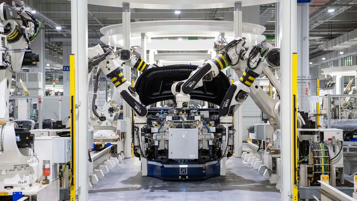
The worldwide stock of operational industrial robots reached a record five million units in 2025, a 9% annual increase.

T-Robotics leads South Korean humanoid robot
T-Robotics is spearheading a national R&D project to develop AI-powered humanoid robots for high-precision display manufacturing, backed by ₩4.5...

Boston Dynamics Opens Atlas Robot Training Center at Hyundai
Boston Dynamics has opened a permanent Robotics Metaplant Application Center at Hyundai's Georgia auto plant to train its Atlas humanoid robots for

OLogic CEO to Present on Robots Learning from Human Demos
OLogic CEO Ted Larson will lead a session on egocentric robot learning at RoboBusiness 2026, exploring how robots can acquire skills from human

Agility Robotics Unveils Digit 5 Humanoid for Factory Floors
Agility Robotics has launched Digit 5, a new humanoid robot designed for manufacturing and logistics. The robot features upgraded legs, batteries...

Vention opens Montreal lab to train AI with factory data
Vention has opened a Physical AI Lab in Montreal to develop robotic manipulation models using data from hundreds of robot cells it deploys annually.